Excel Tips and Tricks / Business Reporting Question: How do I return the rank of a number in a list of numbers relative to other values in a list?

Answer: By using the RANK function in Excel. The function returns the rank of a number in a list of numbers. The rank of a number is its size relative to other values in a list. (If you were to sort the list, the rank of the number would be its position.)

Why: To rank numbers in a given list so that one can easily determine the top performing product

Applies To: Excel (2010, 2007, and 2003):

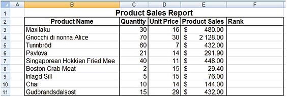
1. Refer to the data given below:

2. Select cell F3 and type; =Rank(E3,$E$3:$E$11)

RANK(number,ref,[order])

The RANK function syntax has the following arguments (argument: A value that provides information to an action, an event, a method, a property, a function, or a procedure.):

Number (Required.) The number whose rank you want to find.

Ref (Required.) An array of, or a reference to, a list of numbers. Non-numeric values in ref are ignored.

Order (Optional.) A number specifying how to rank number.

If order is 0 (zero) or omitted, Microsoft Excel ranks number as if ref were a list sorted in descending order.

If order is any non-zero value, Microsoft Excel ranks number as if ref were a list sorted in ascending order.

3. Press Enter and copy the formula down.

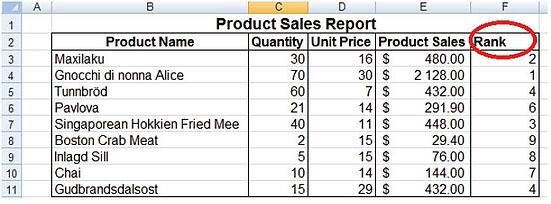
4. The result will be the screen shot below:

The products sales have now being ranked in order of Product Sales Amount, and one can easily determine the best performing product by looking at the rank column and checking the corresponding product name.