---
title: "Excel Tips: PivotTable Calculated Fields"
description: "Business Reporting Question: How can I create my own calculated fields to include in the PivotTable? 

Answer..."
image: https://www.positivevision.biz/hs-fs/file-17316483-jpg/images/excel_tips_-_pivot_calculations_option_1.jpg
---

[![PositiveVision ](https://www.positivevision.biz/hubfs/images/Positive_Vision_Logo_tagline_2015_xsm-1.jpg "Positive_Vision_Logo_tagline_2015_xsm-1")](https://www.positivevision.biz/)

# Business Automation and Software Blog

# Excel Tips: PivotTable Calculated Fields

Posted by [Robert Baran](https://www.positivevision.biz/blog/author/robert-baran) on Fri, Sep 21, 2012 @ 01:44 PM

- [Tweet](https://twitter.com/share)

******Excel Tips and Tricks / Business Reporting Question: ** How can I create my own calculated fields to include in the PivotTable? I intend to have a mark-up of 25% on the sales figure and then calculate the profit.

**Answer: **By using the PivotTable formulae option

**Why: **To create calculated fields

**Applies To MS Excel 2003, 2007, 2010**

**1. **This example is based on last week’s tip on how to create a pivotTable. 

2. Select any cell in the PivotTable.

![Excel Tips and Tricks](https://www.positivevision.biz/hs-fs/file-17316483-jpg/images/excel_tips_-_pivot_calculations_option_1.jpg?width=514&height=124&name=excel_tips_-_pivot_calculations_option_1.jpg)

3. Select as given below:

Excel 2007

![Excel Tips and Tricks](https://www.positivevision.biz/hs-fs/file-17316983-jpg/images/excel_tips_-_pivot_calculations_option_2.jpg?width=597&height=85&name=excel_tips_-_pivot_calculations_option_2.jpg)

Excel 2010

![Excel Tips and Tricks](https://www.positivevision.biz/hs-fs/file-17317424-jpg/images/excel_tips_-_pivot_calculations_option_3.jpg?width=614&height=87&name=excel_tips_-_pivot_calculations_option_3.jpg)

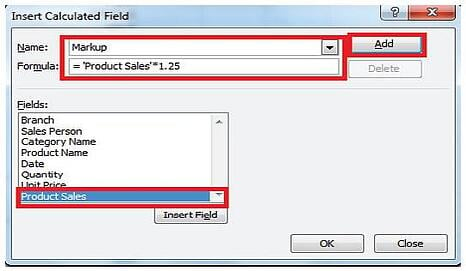
4. The Insert a Calculated field window will open. Enter the following and select add.

![Excel Tips and Tricks](https://www.positivevision.biz/hs-fs/file-17317877-jpg/images/excel_tips_-_pivot_calculations_option_4.jpg?width=466&height=271&name=excel_tips_-_pivot_calculations_option_4.jpg)

5. Rename the field on the PivotTable to Markup (double click on “sum of Markup” field, delete the words “sum of” and press enter).

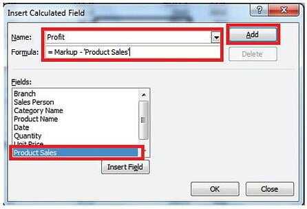
6. Repeat the Process to calculate Profit.

7. Enter the following and select add.

![Excel Tips and Tricks](https://www.positivevision.biz/hs-fs/file-17318250-jpg/images/excel_tips_-_pivot_calculations_option_5.jpg?width=446&height=305&name=excel_tips_-_pivot_calculations_option_5.jpg)

8. Select Ok.

9. Rename the field on the PivotTable to Profit,

10. The result will be as given below.

![Excel Tips   Pivot Calculations Option 6](https://www.positivevision.biz/hs-fs/file-17318495-jpg/images/excel_tips_-_pivot_calculations_option_6.jpg?width=562&height=144&name=excel_tips_-_pivot_calculations_option_6.jpg)

The Markup and Profit figures have been computed by way of adding two calculated fields to the PivotTable.

[![Contact PositiveVision ► ► for a Complimentary  Reporting Consultation](https://no-cache.hubspot.com/cta/default/133208/8610a6e6-e31a-4280-a6e7-b741b3e0dfdb.png)](https://cta-redirect.hubspot.com/cta/redirect/133208/8610a6e6-e31a-4280-a6e7-b741b3e0dfdb)

 Topics: [Business Reporting](https://www.positivevision.biz/blog/topic/business-reporting), [Excel Tips and Tricks](https://www.positivevision.biz/blog/topic/excel-tips-and-tricks)

### Subscribe via Email

### Latest Posts

<https://www.youtube.com/channel/UCWmme9JYZ0Gf6MDQeRXSBww?sub_confirmation=1><https://www.linkedin.com/company/2516562><https://twitter.com/PositiveVision_>

![authorized_solution_partner_w_logo@3x](https://www.positivevision.biz/hs-fs/hubfs/authorized_solution_partner_w_logo@3x.png?width=150&name=authorized_solution_partner_w_logo@3x.png)![Sage Partner Transparent Square](https://www.positivevision.biz/hs-fs/hubfs/Sage%20Partner%20Transparent%20Square.png?width=144&name=Sage%20Partner%20Transparent%20Square.png)    © 2019 PositiveVision • 219 E. Thorndale Ave. Roselle, IL 60172 

800.559.1323 •  [E-mail](mailto:contact@positivevision.biz) • [Privacy Policy](https://www.positivevision.biz/privacy-policy/) • [Sitemap](https://www.positivevision.biz/sitemap/)

 

 

 

 

```json
{
  "@context" : "https://schema.org",
  "@type" : "BlogPosting",
  "author" : {
    "@type" : "Person",
    "name" : "Robert Baran",
    "url" : "https://www.positivevision.biz/blog/author/robert-baran"
  },
  "datePublished" : "2012-09-21T18:44:00.000Z",
  "headline" : "Excel Tips: PivotTable Calculated Fields",
  "image" : [ "https://www.positivevision.biz/hs-fs/file-17316483-jpg/images/excel_tips_-_pivot_calculations_option_1.jpg" ],
  "mainEntityOfPage" : {
    "@id" : "https://www.positivevision.biz/blog/bid/158531/Excel-Tips-PivotTable-Calculated-Fields",
    "@type" : "WebPage"
  },
  "publisher" : {
    "@type" : "Organization",
    "logo" : {
      "@type" : "ImageObject",
      "url" : "None"
    },
    "name" : "PositiveVision"
  }
}
```